Referring Again to the Production Possibilities Curve Answers

2.two The Production Possibilities Bend

Learning Objectives

1. Explicate the concept of the production possibilities curve and understand the implications of its downwards slope and bowed-out shape.
2. Use the production possibilities model to distinguish between full employment and situations of idle factors of production and between efficient and inefficient production.
3. Understand specialization and its relationship to the product possibilities model and comparative advantage.

An economy's factors of production are deficient; they cannot produce an unlimited quantity of appurtenances and services. A production possibilities bend is a graphical representation of the culling combinations of goods and services an economy tin produce. It illustrates the product possibilities model. In cartoon the product possibilities curve, we shall assume that the economy can produce but ii goods and that the quantities of factors of production and the technology bachelor to the economy are fixed.

Constructing a Product Possibilities Curve

To construct a production possibilities curve, we will begin with the case of a hypothetical firm, Alpine Sports, Inc., a specialized sports equipment manufacturer. Christie Ryder began the business fifteen years ago with a single ski production facility near Killington ski resort in central Vermont. Ski sales grew, and she too saw demand for snowboards rising—particularly after snowboard competition events were included in the 2002 Winter Olympics in Salt Lake City. She added a second plant in a nearby town. The second plant, while smaller than the first, was designed to produce snowboards every bit well as skis. She likewise modified the first plant so that it could produce both snowboards and skis. Two years later she added a third plant in another town. While even smaller than the second found, the third was primarily designed for snowboard production but could also produce skis.

Nosotros tin can remember of each of Ms. Ryder's three plants as a miniature economy and analyze them using the production possibilities model. We assume that the factors of production and technology bachelor to each of the plants operated by Alpine Sports are unchanged.

Suppose the first plant, Plant ane, tin produce 200 pairs of skis per month when information technology produces only skis. When devoted solely to snowboards, it produces 100 snowboards per calendar month. It can produce skis and snowboards simultaneously too.

The table in Effigy 2.ii "A Production Possibilities Curve" gives three combinations of skis and snowboards that Plant one can produce each month. Combination A involves devoting the plant entirely to ski production; combination C means shifting all of the plant'southward resources to snowboard production; combination B involves the production of both goods. These values are plotted in a product possibilities curve for Plant ane. The curve is a downward-sloping straight line, indicating that there is a linear, negative relationship between the product of the 2 goods.

Neither skis nor snowboards is an independent or a dependent variable in the production possibilities model; we tin assign either i to the vertical or to the horizontal axis. Here, we have placed the number of pairs of skis produced per month on the vertical axis and the number of snowboards produced per month on the horizontal axis.

The negative slope of the production possibilities curve reflects the scarcity of the plant's upper-case letter and labor. Producing more snowboards requires shifting resources out of ski production and thus producing fewer skis. Producing more than skis requires shifting resource out of snowboard production and thus producing fewer snowboards.

The slope of Plant 1'southward product possibilities curve measures the rate at which Alpine Sports must surrender ski production to produce boosted snowboards. Because the production possibilities bend for Plant one is linear, nosotros can compute the slope between any two points on the curve and get the same issue. Betwixt points A and B, for case, the gradient equals −two pairs of skis/snowboard (equals −100 pairs of skis/50 snowboards). (Many students are helped when told to read this result every bit "−ii pairs of skis per snowboard.") Nosotros go the same value between points B and C, and between points A and C.

Figure two.ii A Product Possibilities Bend

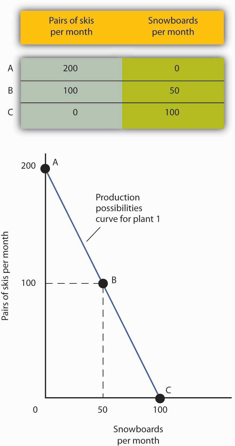
The table shows the combinations of pairs of skis and snowboards that Plant one is capable of producing each month. These are also illustrated with a production possibilities curve. Notice that this curve is linear.

To encounter this relationship more clearly, examine Effigy 2.3 "The Gradient of a Product Possibilities Curve". Suppose Constitute 1 is producing 100 pairs of skis and 50 snowboards per month at betoken B. At present consider what would happen if Ms. Ryder decided to produce one more than snowboard per month. The segment of the bend around bespeak B is magnified in Effigy 2.3 "The Slope of a Production Possibilities Curve". The slope betwixt points B and B′ is −two pairs of skis/snowboard. Producing 1 additional snowboard at point B′ requires giving up 2 pairs of skis. Nosotros tin think of this as the opportunity cost of producing an additional snowboard at Establish 1. This opportunity cost equals the accented value of the slope of the production possibilities curve.

Figure 2.3 The Slope of a Product Possibilities Curve

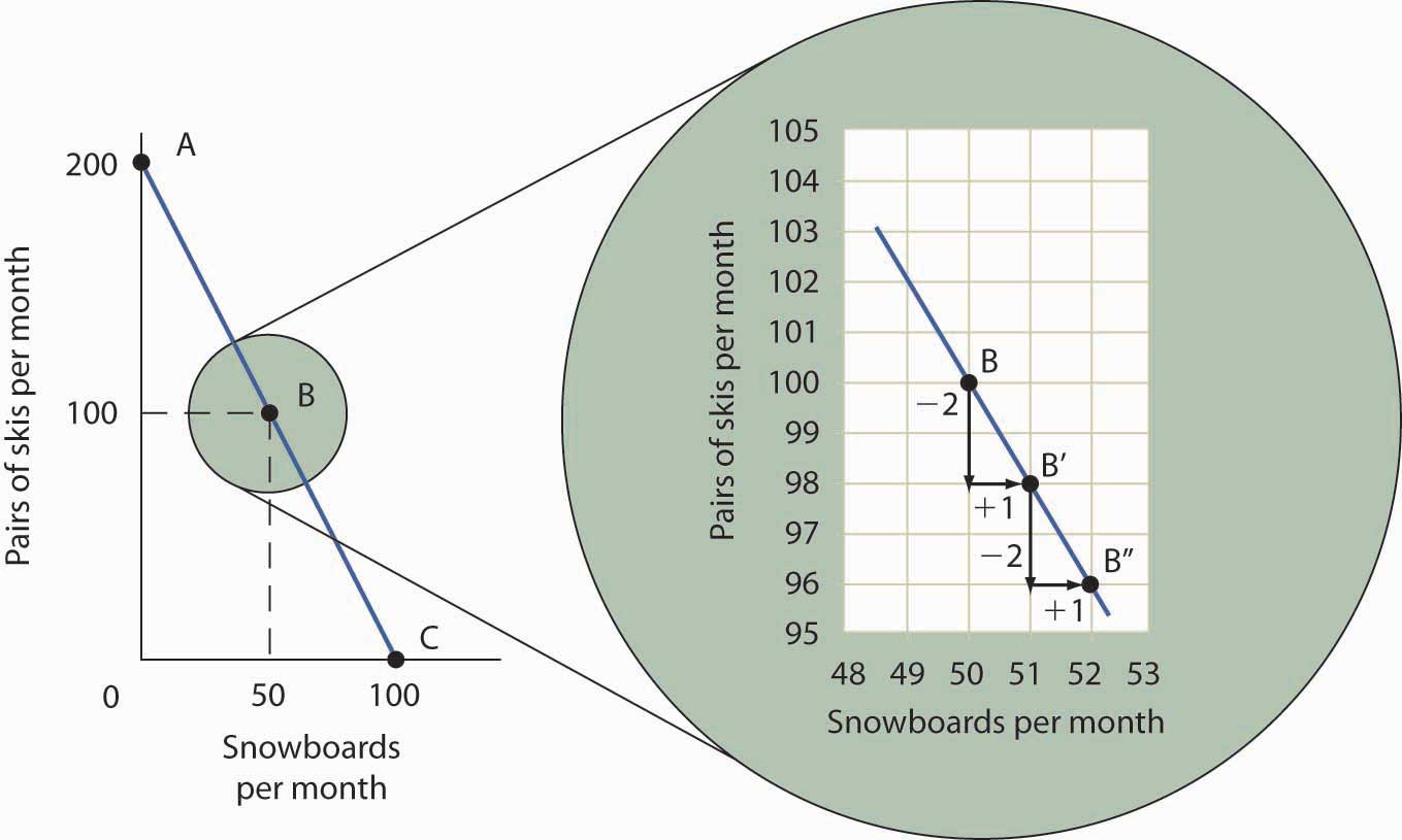
The slope of the linear production possibilities curve in Figure 2.two "A Production Possibilities Curve" is constant; it is −2 pairs of skis/snowboard. In the section of the curve shown hither, the slope can be calculated between points B and B′. Expanding snowboard production to 51 snowboards per calendar month from 50 snowboards per month requires a reduction in ski production to 98 pairs of skis per month from 100 pairs. The slope equals −2 pairs of skis/snowboard (that is, it must requite up 2 pairs of skis to gratuitous upward the resources necessary to produce 1 additional snowboard). To shift from B′ to B″, Alpine Sports must surrender two more than pairs of skis per snowboard. The absolute value of the slope of a product possibilities curve measures the opportunity cost of an additional unit of measurement of the good on the horizontal axis measured in terms of the quantity of the good on the vertical axis that must be forgone.

The absolute value of the slope of any production possibilities curve equals the opportunity cost of an additional unit of the good on the horizontal axis. It is the amount of the good on the vertical centrality that must be given up in order to free up the resources required to produce one more unit of the good on the horizontal axis. We will make employ of this important fact as we proceed our investigation of the production possibilities curve.

Figure 2.4 "Production Possibilities at Three Plants" shows product possibilities curves for each of the house'south iii plants. Each of the plants, if devoted entirely to snowboards, could produce 100 snowboards. Plants ii and 3, if devoted exclusively to ski production, can produce 100 and 50 pairs of skis per calendar month, respectively. The showroom gives the slopes of the production possibilities curves for each plant. The opportunity cost of an additional snowboard at each plant equals the absolute values of these slopes (that is, the number of pairs of skis that must be given up per snowboard).

Figure 2.four Production Possibilities at 3 Plants

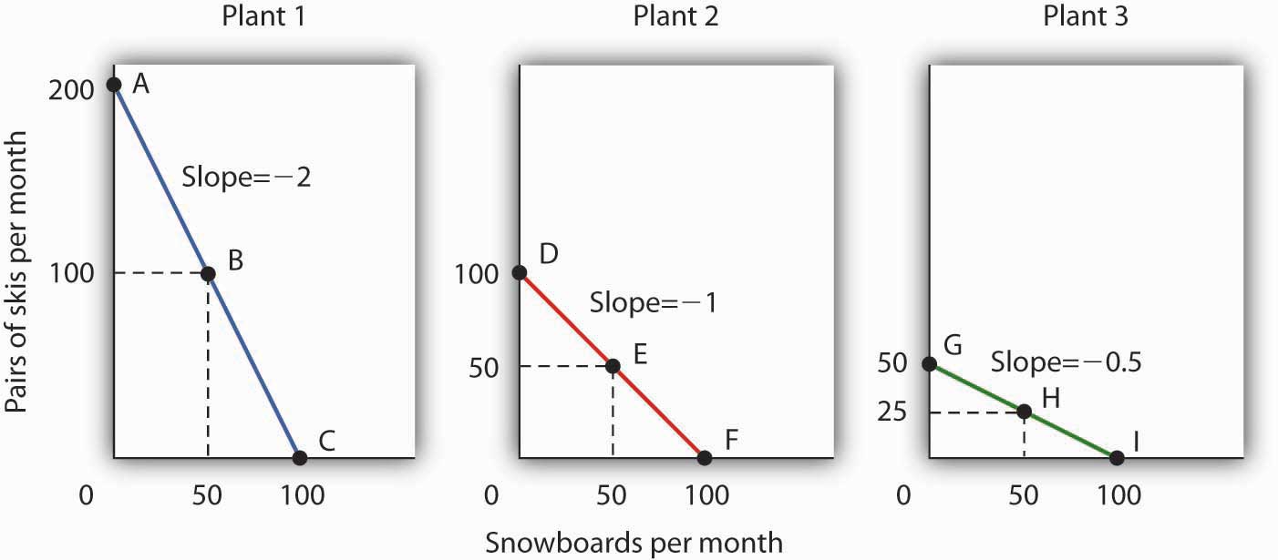
The slopes of the production possibilities curves for each found differ. The steeper the curve, the greater the opportunity cost of an additional snowboard. Hither, the opportunity toll is everyman at Found three and greatest at Establish ane.

The exhibit gives the slopes of the production possibilities curves for each of the firm's iii plants. The opportunity cost of an additional snowboard at each constitute equals the accented values of these slopes. More than generally, the absolute value of the gradient of any production possibilities bend at whatever bespeak gives the opportunity cost of an additional unit of the good on the horizontal axis, measured in terms of the number of units of the good on the vertical axis that must exist forgone.

The greater the absolute value of the slope of the production possibilities curve, the greater the opportunity cost will exist. The plant for which the opportunity cost of an boosted snowboard is greatest is the plant with the steepest production possibilities curve; the plant for which the opportunity toll is lowest is the plant with the flattest product possibilities curve. The constitute with the lowest opportunity cost of producing snowboards is Plant 3; its slope of −0.five means that Ms. Ryder must give up one-half a pair of skis in that institute to produce an additional snowboard. In Plant two, she must surrender one pair of skis to proceeds 1 more snowboard. We have already seen that an boosted snowboard requires giving up two pairs of skis in Plant 1.

Comparative Reward and the Production Possibilities Curve

To construct a combined production possibilities bend for all three plants, we can begin by asking how many pairs of skis Alpine Sports could produce if it were producing only skis. To find this quantity, we add up the values at the vertical intercepts of each of the production possibilities curves in Effigy 2.iv "Production Possibilities at Iii Plants". These intercepts tell us the maximum number of pairs of skis each establish tin produce. Plant ane can produce 200 pairs of skis per calendar month, Plant 2 tin produce 100 pairs of skis at per calendar month, and Constitute iii can produce 50 pairs. Alpine Sports tin can thus produce 350 pairs of skis per month if it devotes its resources exclusively to ski production. In that case, it produces no snowboards.

Now suppose the business firm decides to produce 100 snowboards. That will require shifting ane of its plants out of ski production. Which one will it choose to shift? The sensible matter for it to do is to cull the institute in which snowboards have the lowest opportunity toll—Plant iii. It has an advantage not because it can produce more snowboards than the other plants (all the plants in this case are capable of producing up to 100 snowboards per month) but because it is the to the lowest degree productive plant for making skis. Producing a snowboard in Plant 3 requires giving upward merely half a pair of skis.

Economists say that an economic system has a comparative advantage in producing a good or service if the opportunity toll of producing that good or service is lower for that economy than for any other. Constitute 3 has a comparative reward in snowboard production because it is the plant for which the opportunity cost of additional snowboards is lowest. To put this in terms of the production possibilities curve, Plant 3 has a comparative advantage in snowboard production (the good on the horizontal axis) because its production possibilities bend is the flattest of the iii curves.

Effigy 2.5 The Combined Production Possibilities Curve for Alpine Sports

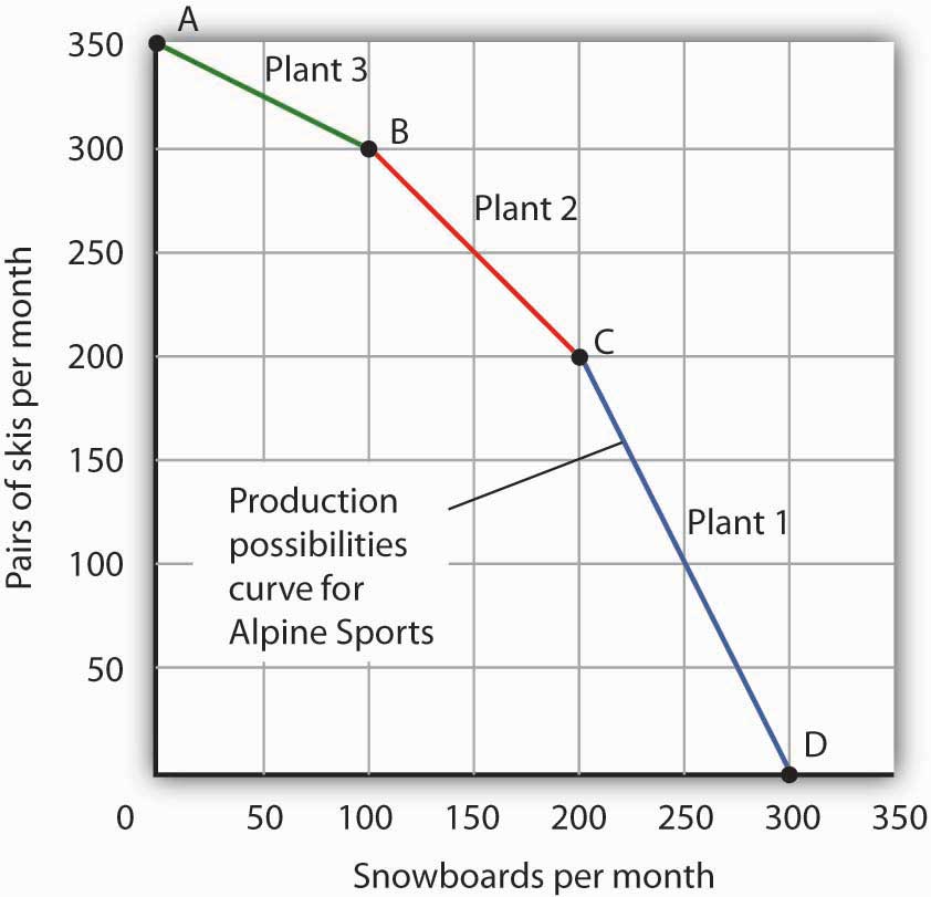
The bend shown combines the production possibilities curves for each plant. At signal A, Alpine Sports produces 350 pairs of skis per month and no snowboards. If the business firm wishes to increase snowboard product, it will first employ Institute 3, which has a comparative reward in snowboards.

Institute three's comparative reward in snowboard product makes a crucial point nigh the nature of comparative advantage. It demand non imply that a particular constitute is especially skillful at an activity. In our example, all three plants are equally practiced at snowboard product. Plant 3, though, is the least efficient of the three in ski production. Tall thus gives up fewer skis when information technology produces snowboards in Plant 3. Comparative advantage thus can stem from a lack of efficiency in the production of an culling skilful rather than a special proficiency in the production of the offset practiced.

The combined production possibilities curve for the firm'south three plants is shown in Figure 2.5 "The Combined Production Possibilities Bend for Alpine Sports". We begin at point A, with all three plants producing only skis. Product totals 350 pairs of skis per month and zero snowboards. If the firm were to produce 100 snowboards at Constitute 3, ski production would fall past 50 pairs per month (recall that the opportunity toll per snowboard at Plant iii is half a pair of skis). That would bring ski production to 300 pairs, at point B. If Alpine Sports were to produce still more than snowboards in a unmarried calendar month, information technology would shift production to Constitute 2, the facility with the next-everyman opportunity cost. Producing 100 snowboards at Constitute 2 would leave Alpine Sports producing 200 snowboards and 200 pairs of skis per calendar month, at point C. If the firm were to switch entirely to snowboard production, Establish 1 would be the last to switch because the cost of each snowboard at that place is 2 pairs of skis. With all three plants producing simply snowboards, the firm is at indicate D on the combined production possibilities curve, producing 300 snowboards per month and no skis.

Notice that this production possibilities bend, which is made up of linear segments from each assembly constitute, has a bowed-out shape; the absolute value of its slope increases as Alpine Sports produces more and more snowboards. This is a result of transferring resources from the production of one adept to another according to comparative advantage. We shall examine the significance of the bowed-out shape of the curve in the next section.

The Police of Increasing Opportunity Price

We see in Figure 2.5 "The Combined Production Possibilities Bend for Alpine Sports" that, beginning at point A and producing only skis, Tall Sports experiences higher and higher opportunity costs equally information technology produces more snowboards. The fact that the opportunity toll of additional snowboards increases as the firm produces more of them is a reflection of an important economic law. The law of increasing opportunity toll holds that as an economy moves along its production possibilities bend in the direction of producing more of a particular practiced, the opportunity cost of boosted units of that skillful will increase.

We accept seen the police of increasing opportunity toll at work traveling from point A toward point D on the production possibilities curve in Effigy 2.5 "The Combined Production Possibilities Curve for Tall Sports". The opportunity price of each of the outset 100 snowboards equals half a pair of skis; each of the next 100 snowboards has an opportunity price of i pair of skis, and each of the concluding 100 snowboards has an opportunity cost of 2 pairs of skis. The law also applies equally the firm shifts from snowboards to skis. Suppose it begins at point D, producing 300 snowboards per month and no skis. It can shift to ski production at a relatively depression cost at commencement. The opportunity price of the starting time 200 pairs of skis is just 100 snowboards at Institute 1, a movement from bespeak D to point C, or 0.v snowboards per pair of skis. We would say that Plant 1 has a comparative reward in ski production. The side by side 100 pairs of skis would be produced at Establish 2, where snowboard product would fall by 100 snowboards per calendar month. The opportunity cost of skis at Plant two is one snowboard per pair of skis. Institute iii would be the final plant converted to ski production. There, 50 pairs of skis could be produced per month at a cost of 100 snowboards, or an opportunity cost of 2 snowboards per pair of skis.

The bowed-out production possibilities curve for Alpine Sports illustrates the law of increasing opportunity price. Scarcity implies that a production possibilities bend is downward sloping; the constabulary of increasing opportunity cost implies that it will be bowed out, or concave, in shape.

The bowed-out curve of Figure ii.5 "The Combined Production Possibilities Curve for Tall Sports" becomes smoother equally we include more than production facilities. Suppose Alpine Sports expands to 10 plants, each with a linear production possibilities curve. Panel (a) of Figure 2.6 "Production Possibilities for the Economy" shows the combined curve for the expanded firm, synthetic every bit we did in Figure ii.5 "The Combined Production Possibilities Curve for Alpine Sports". This production possibilities curve includes 10 linear segments and is near a smooth curve. As we include more and more production units, the bend volition go smoother and smoother. In an actual economy, with a tremendous number of firms and workers, it is easy to see that the production possibilities curve volition be smooth. Nosotros volition generally describe product possibilities curves for the economy every bit smooth, bowed-out curves, similar the one in Panel (b). This production possibilities curve shows an economy that produces merely skis and snowboards. Discover the curve still has a bowed-out shape; it still has a negative slope. Notice too that this curve has no numbers. Economists often employ models such as the production possibilities model with graphs that bear witness the full general shapes of curves but that practice not include specific numbers.

Effigy ii.half dozen Production Possibilities for the Economic system

As we combine the production possibilities curves for more and more than units, the curve becomes smoother. It retains its negative slope and bowed-out shape. In Panel (a) nosotros take a combined product possibilities bend for Alpine Sports, assuming that it now has 10 plants producing skis and snowboards. Even though each of the plants has a linear curve, combining them according to comparative reward, equally nosotros did with 3 plants in Figure ii.v "The Combined Production Possibilities Curve for Alpine Sports", produces what appears to exist a smooth, nonlinear curve, fifty-fifty though it is made up of linear segments. In drawing production possibilities curves for the economy, we shall by and large assume they are smooth and "bowed out," equally in Console (b). This curve depicts an entire economy that produces simply skis and snowboards.

Movements Along the Production Possibilities Bend

We can use the production possibilities model to examine choices in the production of appurtenances and services. In applying the model, nosotros assume that the economy can produce two goods, and nosotros assume that technology and the factors of production available to the economy remain unchanged. In this section, we shall assume that the economy operates on its production possibilities bend so that an increase in the production of one proficient in the model implies a reduction in the product of the other.

We shall consider 2 appurtenances and services: national security and a category nosotros shall telephone call "all other goods and services." This 2nd category includes the unabridged range of goods and services the economy tin can produce, bated from national defense and security. Clearly, the transfer of resource to the effort to enhance national security reduces the quantity of other goods and services that can be produced. In the wake of the 9/xi attacks in 2001, nations throughout the earth increased their spending for national security. This spending took a diverseness of forms. One, of course, was increased defence spending. Local and land governments also increased spending in an effort to preclude terrorist attacks. Airports around the world hired additional agents to inspect baggage and passengers.

The increase in resources devoted to security meant fewer "other appurtenances and services" could exist produced. In terms of the production possibilities curve in Effigy 2.7 "Spending More for Security", the choice to produce more security and less of other goods and services means a movement from A to B. Of class, an economy cannot actually produce security; it can but attempt to provide it. The attempt to provide it requires resource; it is in that sense that we shall speak of the economy every bit "producing" security.

Figure 2.7 Spending More for Security

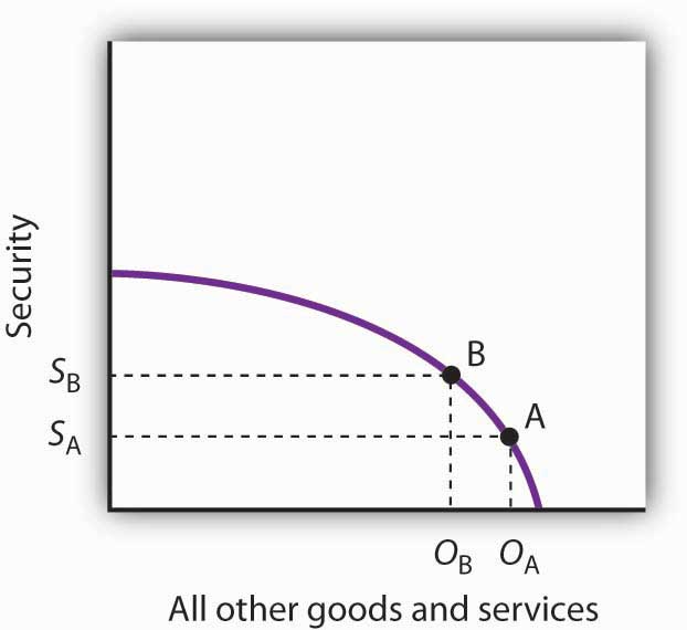
Here, an economic system that can produce 2 categories of goods, security and "all other goods and services," begins at point A on its production possibilities curve. The economy produces S _A units of security and O _A units of all other goods and services per menses. A movement from A to B requires shifting resources out of the production of all other goods and services and into spending on security. The increase in spending on security, to S _A units of security per flow, has an opportunity cost of reduced product of all other goods and services. Production of all other goods and services falls past O _A – O _B units per period.

At bespeak A, the economic system was producing Due south _A units of security on the vertical axis—defense force services and diverse forms of police protection—and O _A units of other appurtenances and services on the horizontal axis. The decision to devote more than resources to security and less to other goods and services represents the pick we discussed in the chapter introduction. In this case we have categories of goods rather than specific goods. Thus, the economy chose to increase spending on security in the endeavor to defeat terrorism. Since nosotros accept assumed that the economy has a fixed quantity of available resources, the increased use of resources for security and national defense force necessarily reduces the number of resources available for the production of other appurtenances and services.

The police force of increasing opportunity cost tells usa that, as the economy moves along the production possibilities curve in the management of more of ane good, its opportunity cost will increase. We may conclude that, as the economic system moved along this curve in the management of greater production of security, the opportunity cost of the additional security began to increase. That is because the resources transferred from the product of other goods and services to the production of security had a greater and greater comparative reward in producing things other than security.

The product possibilities model does non tell u.s. where on the curve a particular economy will operate. Instead, it lays out the possibilities facing the economy. Many countries, for case, chose to move forth their respective production possibilities curves to produce more security and national defense and less of all other goods in the wake of 9/11. Nosotros will see in the chapter on demand and supply how choices about what to produce are fabricated in the marketplace.

Producing on Versus Producing Inside the Product Possibilities Curve

An economy that is operating inside its production possibilities bend could, by moving onto it, produce more than of all the appurtenances and services that people value, such as food, housing, pedagogy, medical intendance, and music. Increasing the availability of these goods would better the standard of living. Economists conclude that information technology is amend to be on the product possibilities curve than within information technology.

Two things could go out an economy operating at a betoken within its product possibilities curve. First, the economic system might fail to use fully the resources available to information technology. 2nd, it might not allocate resources on the basis of comparative advantage. In either instance, product within the production possibilities curve implies the economy could improve its performance.

Idle Factors of Production

Suppose an economy fails to put all its factors of production to work. Some workers are without jobs, some buildings are without occupants, some fields are without crops. Considering an economy's production possibilities bend assumes the full use of the factors of production available to it, the failure to apply some factors results in a level of production that lies within the production possibilities curve.

If all the factors of production that are available for utilize under current market weather condition are beingness utilized, the economy has achieved full employment. An economy cannot operate on its production possibilities curve unless it has full employment.

Effigy 2.eight Idle Factors and Production

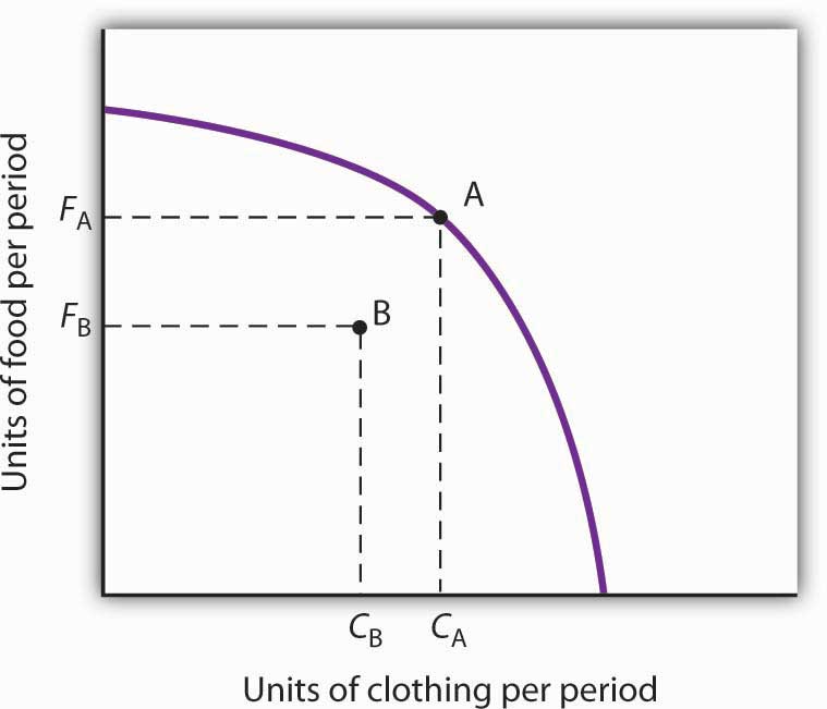
The production possibilities curve shown suggests an economy that tin produce two goods, food and clothing. As a effect of a failure to achieve full employment, the economy operates at a point such as B, producing F _B units of food and C _B units of clothing per period. Putting its factors of product to work allows a motion to the production possibilities curve, to a point such as A. The product of both appurtenances rises.

Figure ii.8 "Idle Factors and Production" shows an economy that tin can produce nutrient and clothing. If it chooses to produce at bespeak A, for example, it can produce F _A units of nutrient and C _A units of clothing. At present suppose that a big fraction of the economy'southward workers lose their jobs, so the economy no longer makes full use of one cistron of product: labor. In this example, production moves to betoken B, where the economy produces less food (F _B) and less clothing (C _B) than at point A. Nosotros often think of the loss of jobs in terms of the workers; they have lost a chance to work and to earn income. But the production possibilities model points to some other loss: appurtenances and services the economic system could have produced that are not being produced.

Inefficient Production

Now suppose Alpine Sports is fully employing its factors of production. Could it still operate inside its production possibilities bend? Could an economy that is using all its factors of production still produce less than it could? The answer is "Yes," and the fundamental lies in comparative advantage. An economy achieves a signal on its production possibilities curve only if it allocates its factors of production on the ground of comparative reward. If information technology fails to do that, it will operate within the curve.

Suppose that, as earlier, Alpine Sports has been producing only skis. With all three of its plants producing skis, information technology can produce 350 pairs of skis per calendar month (and no snowboards). The firm then starts producing snowboards. This time, however, imagine that Alpine Sports switches plants from skis to snowboards in numerical order: Plant 1 first, Plant 2 second, and then Plant iii. Figure 2.9 "Efficient Versus Inefficient Product" illustrates the result. Instead of the bowed-out product possibilities curve ABCD, we become a bowed-in bend, AB′C′D. Suppose that Alpine Sports is producing 100 snowboards and 150 pairs of skis at point B′. Had the firm based its production choices on comparative reward, it would take switched Plant three to snowboards and then Establish ii, so it could have operated at a betoken such as C. It would be producing more snowboards and more pairs of skis—and using the aforementioned quantities of factors of production it was using at B′. Had the house based its production choices on comparative advantage, it would have switched Establish iii to snowboards and then Found ii, then information technology would take operated at indicate C. It would be producing more than snowboards and more pairs of skis—and using the aforementioned quantities of factors of production it was using at B′. When an economy is operating on its production possibilities curve, nosotros say that information technology is engaging in efficient production. If information technology is using the same quantities of factors of product but is operating inside its production possibilities curve, it is engaging in inefficient production. Inefficient product implies that the economic system could be producing more goods without using any boosted labor, capital, or natural resources.

Figure 2.nine Efficient Versus Inefficient Production

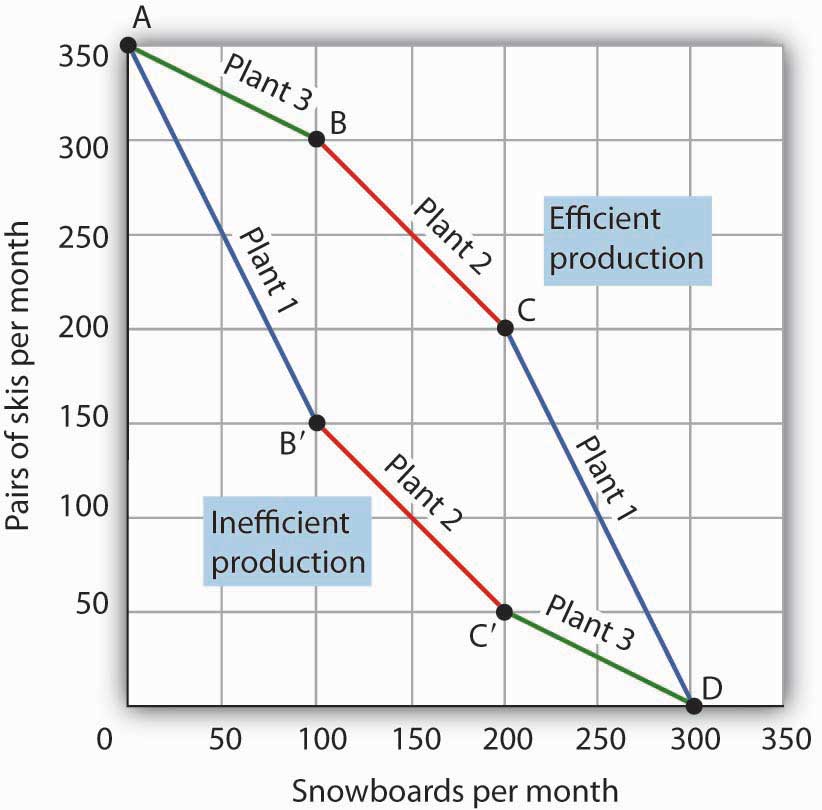
When factors of production are allocated on a basis other than comparative advantage, the outcome is inefficient product. Suppose Alpine Sports operates the three plants we examined in Figure 2.4 "Production Possibilities at Three Plants". Suppose further that all three plants are devoted exclusively to ski product; the firm operates at A. Now suppose that, to increase snowboard production, it transfers plants in numerical order: Plant ane first, then Plant 2, and finally Plant 3. The upshot is the bowed-in curve AB′C′D. Production on the product possibilities curve ABCD requires that factors of product be transferred co-ordinate to comparative advantage.

Points on the product possibilities bend thus satisfy two weather condition: the economy is making full utilize of its factors of production, and it is making efficient use of its factors of product. If there are idle or inefficiently allocated factors of product, the economy volition operate inside the production possibilities curve. Thus, the production possibilities curve non merely shows what tin can be produced; it provides insight into how appurtenances and services should exist produced. It suggests that to obtain efficiency in production, factors of production should be allocated on the ground of comparative advantage. Further, the economy must make full apply of its factors of production if it is to produce the goods and services it is capable of producing.

Specialization

The production possibilities model suggests that specialization will occur. Specialization implies that an economy is producing the goods and services in which it has a comparative advantage. If Tall Sports selects signal C in Figure two.9 "Efficient Versus Inefficient Production", for example, it will assign Plant i exclusively to ski production and Plants 2 and 3 exclusively to snowboard production.

Such specialization is typical in an economic organisation. Workers, for instance, specialize in particular fields in which they have a comparative reward. People work and employ the income they earn to buy—perhaps import—appurtenances and services from people who have a comparative reward in doing other things. The consequence is a far greater quantity of goods and services than would be available without this specialization.

Think virtually what life would be like without specialization. Imagine that yous are suddenly completely cut off from the remainder of the economy. Yous must produce everything you consume; you obtain cypher from anyone else. Would you be able to consume what you consume now? Clearly non. It is difficult to imagine that about of us could even survive in such a setting. The gains we achieve through specialization are enormous.

Nations specialize too. Much of the land in the United States has a comparative advantage in agronomical production and is devoted to that activity. Hong Kong, with its huge population and tiny endowment of land, allocates almost none of its land to agricultural use; that selection would be likewise costly. Its land is devoted largely to nonagricultural use.

Key Takeaways

• A production possibilities curve shows the combinations of ii goods an economy is capable of producing.
• The downwards slope of the product possibilities curve is an implication of scarcity.
• The bowed-out shape of the production possibilities curve results from allocating resources based on comparative advantage. Such an allocation implies that the law of increasing opportunity price will concur.
• An economy that fails to make full and efficient employ of its factors of production will operate inside its production possibilities curve.
• Specialization means that an economy is producing the goods and services in which information technology has a comparative reward.

Endeavor Information technology!

Suppose a manufacturing firm is equipped to produce radios or calculators. It has 2 plants, Establish R and Found S, at which it tin can produce these goods. Given the labor and the capital available at both plants, it can produce the combinations of the ii goods at the 2 plants shown.

Output per day, Plant S
Combination	Calculators	Radios
D	fifty	0
Eastward	25	50
F	0	100

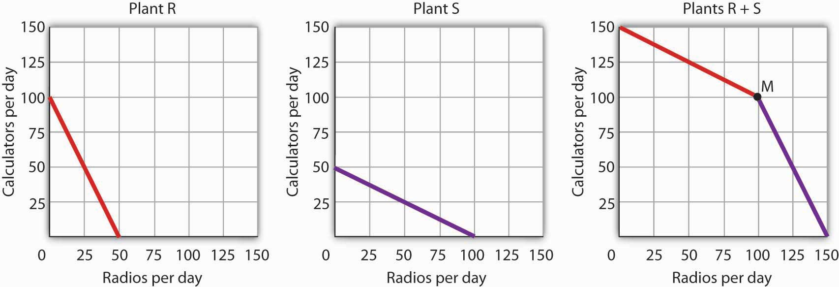
Put calculators on the vertical centrality and radios on the horizontal axis. Draw the production possibilities curve for Institute R. On a separate graph, draw the production possibilities curve for Plant S. Which plant has a comparative reward in calculators? In radios? Now draw the combined curves for the two plants. Suppose the firm decides to produce 100 radios. Where will information technology produce them? How many calculators will it exist able to produce? Where volition it produce the calculators?

Example in Point: The Cost of the Great Low

Figure two.10

The U.S. economic system looked very healthy in the beginning of 1929. It had enjoyed seven years of dramatic growth and unprecedented prosperity. Its resources were fully employed; information technology was operating quite close to its production possibilities curve.

In the summertime of 1929, however, things started going wrong. Product and employment fell. They continued to fall for several years. By 1933, more than 25% of the nation's workers had lost their jobs. Production had plummeted by about 30%. The economy had moved well within its production possibilities curve.

Output began to grow after 1933, but the economy continued to take vast numbers of idle workers, idle factories, and idle farms. These resources were non put dorsum to work fully until 1942, after the U.S. entry into Globe War 2 demanded mobilization of the economy's factors of production.

Between 1929 and 1942, the economy produced 25% fewer appurtenances and services than it would have if its resources had been fully employed. That was a loss, measured in today's dollars, of well over $three trillion. In material terms, the forgone output represented a greater cost than the United States would ultimately spend in World War II. The Not bad Depression was a costly feel indeed.

Answer to Endeavor Information technology! Trouble

The product possibilities curves for the two plants are shown, forth with the combined curve for both plants. Plant R has a comparative advantage in producing calculators. Found S has a comparative advantage in producing radios, and then, if the firm goes from producing 150 calculators and no radios to producing 100 radios, information technology will produce them at Plant S. In the production possibilities curve for both plants, the business firm would be at M, producing 100 calculators at Establish R.

Figure 2.11

valentinodiany1971.blogspot.com

Source: https://open.lib.umn.edu/principleseconomics/chapter/2-2-the-production-possibilities-curve/

Share this post